A New Paradigm for Lossy Media Compression

Introduction
The world has moved toward a more fluid work life where flexibility is the new normal and the demand for quality online communication is more prevalent than ever. Recent times have highlighted the disadvantages faced by users in developing countries and rural areas when trying to access reliable internet. Even in locations with strong internet we struggle to conduct a meeting without interruption.
Quality of audio is a significant factor when it comes to the efficiency with which businesses operate, communicate, and stay connected.
Our media-rich digital experiences are powered behind-the-scenes by audio and video codecs, these aim to reduce the data size of media we consume, saving money on mobile data, reducing the load on the public internet, and overall enabling a much better experience in a variety of network conditions.
In general, classical codecs reduce data size in the order of 10x from the original media. AI-powered codecs (in general) can unlock another ~10x on top of this, enabling around a 100x reduction in data size. We don’t always need such extreme compression, in these cases we can use the extra data savings to mitigate the effects of packet loss on spotty connections, for example.
AI-powered compression schemes are a step-change in media coding technology; providing increasing quality using less data, enabling good-quality voice and video chats on a much wider variety of connections, and moving towards universal access to high-quality media.
Classical Compression Schemes
Classical lossy compression schemes such as JPEG for images and MP3 for music work by removing as much information from the original media as possible, while still retaining the essential components for viewing or listening at an acceptable level of quality. The algorithms behind these codecs use knowledge about the human eyes (psychovisual) and ears (psychoacoustics), in order to remove the information that has the least impact on the ability for a human to perceive the media.
A major limitation of this classical approach is that once information is removed by the sender, it cannot be recovered by the receiver. This is where generative Machine Learning (ML) models offer a solution.
Comparing Vaux to Classical Audio Compression Schemes
Here we demonstrate a quick comparison between Vaux, Opus and MP3 given a noisy input file. These audios have a sample rate of 16kHz.
For more audio samples and comparisons, listen to the demo on our website.
Core Enabling Technologies
There are two key AI technologies that give rise to the era of AI-powered codecs: AI techniques that learn to extract compact and meaningful representations from media, Representation Learning; and powerful Generative Models that can synthesise natural looking and sounding media from these compact representations.
Generative Models
Generative models are trained over enormous amounts of real world data from a specified domain — images, audio, or text for example. The goal is that the model will be able to generate data similar to what it’s seen during training. The model is forced, by the design of it’s architecture, to discover and efficiently internalise the essence of the media in order to generate new examples.
Modern generative models are capable of creating high-fidelity media, such as images and voice. Take for example OpenAI’s DALL·E work — it is a generative model that synthesises high-fidelity images from text descriptions. The input is a tiny amount of data, a couple of sentences of text, and the output is a high fidelity, intelligible image.
Theoretically, a sender could use an image captioning model to generate a text description of an image. The description is sent to a recipient, who can use something similar to DALL·E to regenerate the image at their end. The bit in the middle, the compressed representation, is only a couple hundred bytes of text used to condition the generative model at the receiving end.
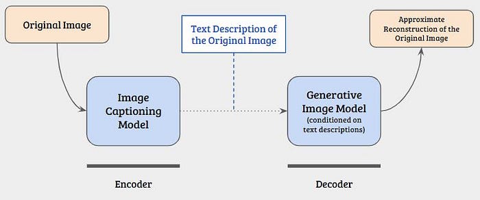
This scheme is analogous to describing a scene to a friend. They have a well-trained idea of what various objects and situations look like. They can use this, combined with (or conditioned on) the description you provide to imagine the image. Ideally they picture something close to what you described, and you didn’t have to explain the colour of every pixel, this is a human-powered lossy compression scheme!
A well-trained generative model can use it’s internal understanding about the media seen during training (just as your friend uses their understanding of what things look like) to synthesise new data (imagine the scene) given a very small number of conditioning parameters (the description you gave them).
Representation Learning
Autoencoders are one example of representation learning techniques. They leverage neural networks to learn a compact, yet rich and meaningful representation of the input media. The autoencoder architecture consists of an encoder and a decoder, with an information bottleneck imposed between the two, the bottleneck forces the compressed representation to be extracted from the input.
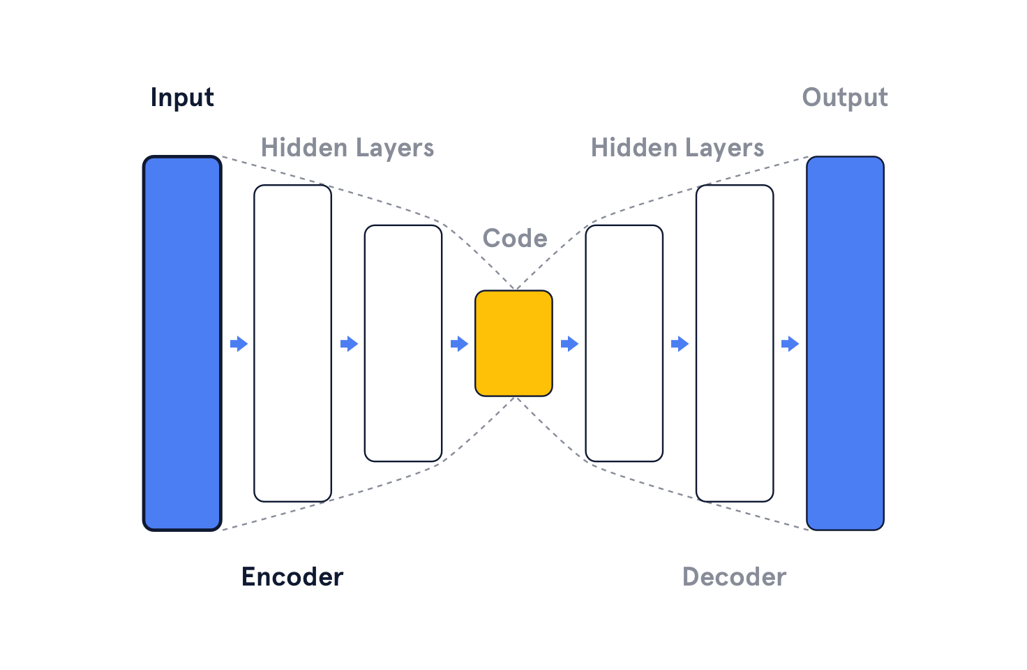
The input to the encoder is a set of features that represent the raw data, this could be pixel values of an image or a series of audio samples. The encoder compresses these features into a smaller representation called the code, embedding, or latent. The decoder tries to reconstruct the original input from this latent.
During training, the encoder learns a better way to represent the essence of the input in it’s latent representation; and the decoder learns how to best ‘imagine’ the details of the original input in order to reconstruct it.
This technique assumes that there is redundancy in the input data which the autoencoder exploits to keep only features that are essential for reconstruction at the decoder.
Vaux Architecture
The Vaux denoising and compression pipeline brings together a handful of modern deep learning techniques. A time-domain denoising model, a recurrent autoencoder with feedback and a hybrid neural network and Digital Signal Processing (DSP) vocoder.

The Vaux compression model works on 10ms frames of audio. Each frame can be represented by 16bits, which equates to a data rate of 1.6kbps. The decoder takes these frames and predicts parameters for a DSP-based vocoder, the vocoder synthesises audio using these parameters.
A 16kHz uncompressed .wav file has a data rate of 256kbps. Encoded with Vaux, the same file can be compressed to 1.6kbps, a 160x reduction in data size. To achieve a comparable level of quality using Opus requires a bitrate of 16–20kbps, only a 16x size reduction from the original media.
Now we’ll get into the details about each module in our architecture, this gets quite technical! Feel free to skip to the end for our development roadmap, or for details about how to follow our journey.
Denoising
Denoising is the task of un-mixing two signals, a speech signal which we want to keep and a noise signal which we want to discard. This task is essentially the same as blind speaker separation for which there is a wealth of research available among the Deep Learning community. At Vaux we have implemented and trained our own version of ConvTASNet, a speaker separation model that has achieved State-Of-The-Art (SOTA) results.
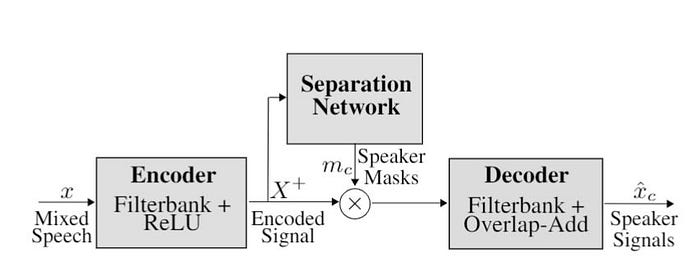
ConvTASNet has a learned filter-bank at it’s input, splitting the input audio into many frequency bands. For each frequency band a neural network predicts a mask that is applied to the audio in that band, attenuating the noise. Each mask network can specialise within it’s frequency band, as there are different types of noise at low frequencies compared to high frequencies. When no noise is detected the ConvTASNet has no effect on the audio passing through. The masked signals from each band are recombined back into one signal using an inverse filterbank.
We’ve found that denoising is a critical pre-processing step before compression. The denoising process can be thought of as bringing noisy audio from the real-world closer to the distribution of audio seen during training, increasing the performance of the encoder and decoder dramatically.
Feedback Recurrent Auto Encoder
The Vaux encoder/decoder architecture is based on the Feedback Recurrent Auto Encoder (FRAE), proposed in this paper from Qualcomm. This work introduces a recurrent autoencoder scheme, where the hidden state of the encoder and decoder are shared.
FRAE enables a more compact latent representation than a separate-recurrence scheme. The shared hidden state encodes a summary of the frames seen so far. The encoder uses the hidden state to encode a latent that only contains the residual information the decoder will need to reconstruct the next frame from the combination of the hidden state and the latent encoding.
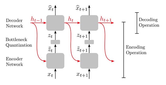
This architecture lends itself well to the task of compression as only a small amount of information (the latent) needs to be transmitted from the sender to receiver, given both can compute their own copies of the hidden state. On the sender side the decoder is run for each frame of the encoding process to update the hidden state. Note that this doesn’t require synthesising the frame back to audio so this isn’t a large computational cost.
The encoder operates over Mel-spectrogram frames. Each frame contains a frequency domain representation of a 10ms slice of the input audio. These 10ms frames are passed through the encoder, a Gated Recurrent Unit (GRU), to produce a small latent vector per frame. This vector is quantised using a scalar quantisation technique with a small codebook.
At this point the quantised vectors can be concatenated and stored, or transmitted to a receiver as a bitstream.
For the decoding process the quantised vector is de-quantised, as the decoder has the same copy of the learned codebook. The decoder is a similar model to the encoder except it transforms the small latent vector into a larger vector of parameters for the vocoder.
These parameters include a set of amplitudes for a harmonic oscillator and filter-band coefficients for a filtered noise generator.
Vocoder
Vaux has developed a Differential Digital Signal Processing (DDSP) vocoder, based on the DDSP work published by Google Magenta.
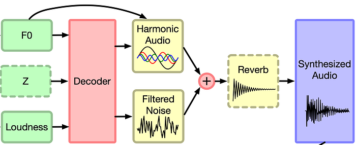
The rationale behind DDSP is to combine the interpretability of basic DSP elements, such as oscillators and filters, with the expressivity of deep learning. Simple and interpretable, DSP elements can be used to create complex realistic signals, such as human speech, by controlling their many parameters on a small time scale. A set of sinusoidal oscillators and linear filters can be combined to synthesise natural-sounding human speech when the frequencies and filter parameters are tuned in just the right way. It is difficult, or impossible, to do this by hand, which is where ML provides a solution.
At every 10ms frame the decoder is outputting a set of parameters for the DDSP modules and these are selected by the decoder to best synthesise that frame back into audio. By utilising DDSP we relieve the decoder of the computationally expensive task of modelling the relationship between thousands of time-domain audio samples and instead give it the much simpler and more human-interpretable task of selecting DSP parameters.
Note About Compute Costs
One concern about ML powered compression, is that ML models are generally known for their high computational requirements, and mostly require expensive accelerators like GPUs. It’s interesting to think about ML powered compression as trading network bandwidth for local compute power. We’ve worked to avoid this issue by selecting ML architectures that are computationally light, or can be made computationally light using techniques like pruning, removing the need for a high-power accelerator like a GPU.
The Vaux denoising and compression pipeline can run many times faster than real-time on a single laptop-grade CPU core. This performance represents the lower-limit of what Vaux will eventually achieve, as the Vaux pipeline is mostly in a development state and hasn’t yet seen the benefits of moving to high-performance production frameworks and inference techniques.
Development Roadmap
Variable Bit Rate
While we’ve achieved great results so far with the models described above, we are exploring a technique that will allow Vaux to operate in a Variable Bit Rate (VBR) mode. This technique will remove the need for quantisation, which is currently a source of artefacts in the output audio.
As far as we know, Vaux will be the first practical implementation of a learned variable bitrate code. We can use the extra bandwidth savings from our VBR scheme to help mitigate packet loss, enabling wideband speech across low-bandwidth and spotty connections.
Vocoder Upgrade
We are moving to real-time WaveRNN vocoder, while not as interpretable as our current DDSP vocoder it is generating higher fidelity audio, and removes the need for accurate pitch-tracking. Extracting accurate pitch values from real-world audio has been a limitation to robust generalisation for our DDSP vocoder. A vocoder with less ‘moving parts’ enables us to achieve better generalisation to any voice in any environment.
Follow Our Journey!
Our next demo will incorporate VBR, our new vocoder, and feature more real-world comparisons; and our next update will include details about our beta product!
Signup to our mailing list to be the first to hear about our progress.
Feel free to reach out to our team directly:
CEO — steph@vaux.io
CTO — lindsay@vaux.io